Designing Reinforcement Learning Agents

In this month, the work was mainly devoted to mitigating the sample efficiency problem of Reinforcement Learning. However, the first days were spent integrating the LogiTech steering wheel and pedals in CARLA and fixing unexpected crashes of the simulator.

CARLA

LogiTech

Since the main objective of this Ph.D. is to combine Imitation Learning (IL) and Reinforcement Learning (RL), it is mandatory create an interface where the humans can provide the demonstrations. For that, we integrated the LogitTech steering wheel and pedals in CARLA (issue #6):

Unexpected CARLA Server crashes

After implementing all infrastructure related with CARLA, I tried to run a simple RL agent over 10^6 steps. However, the CARLA Server was crashing after 30/40k steps:

Signal 11 caught.
Malloc Size=65538 LargeMemoryPoolOffset=65554
4.26.2-0+++UE4+Release-4.26 522 0
Disabling core dumps.
CommonUnixCrashHandler: Signal=11
Engine crash handling finished; re-raising signal 11 for the default handler. Good bye.
./CarlaUE4.sh: line 5: 13 Segmentation fault (core dumped) "$UE4_PROJECT_ROOT/CarlaUE4/Binaries/Linux/CarlaUE4-Linux-Shipping" CarlaUE4 "$@"


After several unsuccessful attempts to find the the cause of the error, I downgraded CARLA version from 0.9.13 to 0.9.10.1 and the problem was solved (issue #29).

Reinforcement Learning

Sample Efficiency

Reinforcement Learning is known to be sample inefficient, that is, it needs a lot of samples to learn. This problem is even more evident when using high dimensional inputs as is the case of images. A number of approaches have been proposed to mitigate this problem (sorted by ascending order of effectiveness):

1. Data augmentation: paper
2. Auto Encoder: paper
3. Contrastive Learning: paper
4. DDPG with sigma decaying: paper

These techniques are meant to be included in a generic architecture composed of an image encoder followed by a Deep RL algorithm. To start, I decided to implement RegNet as image encoder and then Soft Actor Critic as the deep RL algorithm.

Regnet followed by SAC

The architecture of this agent is the following:

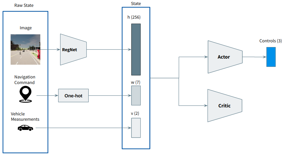
The navigation command is a high-level indication provided by the global planner. Examples include "go straight" and "turn left". This information is conveyed into the network using one-hot encoding. In the future, this will be replaced by a fully-conected network that receives the next n waypoints and outputs a feature vector of m elements. In addiction to the navigation comand, we are also taking in consideration 2 elements: current velocity normalized between 0 and 1, and the current steering angle.

This system was tested in CARLA, and the results were embarrassingly bad (issue #17):


The cause of this behavior was improper exploration. The exploration of the agent consists in generating random values for the throttle, steer and braking. However, by generating random values the car will never start moving because for the car to start to move, the throttle must be pressed for some seconds while leaving the brake untouched.

RegNet followed by SAC with longitudinal controller

To overcome the trottle/brake issue, we decided to change the outputs of the agent to steering angle and predicted speed, and then implement a PID controller to convert the predicted speed into throttle and brake commands (issue #18). The architecture of the system was then change to:

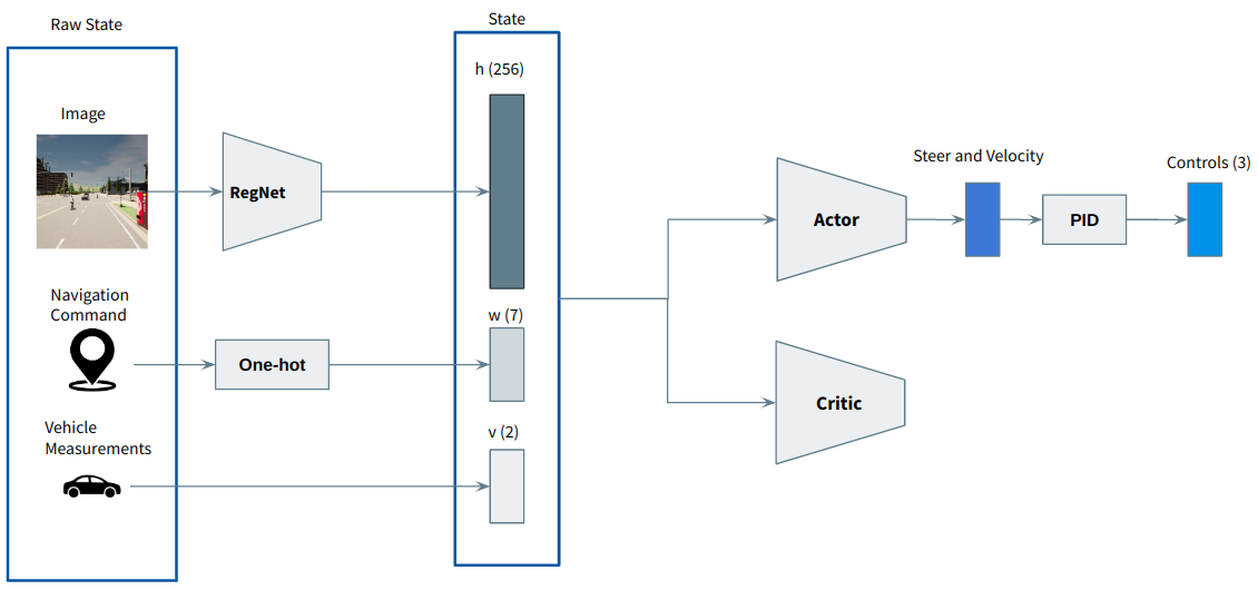
And the curve of the PID (kp=1.0, ki=0.2, kd=0.001) when setting desired speed to 6 m/s was the following (1 step = 0.1s):
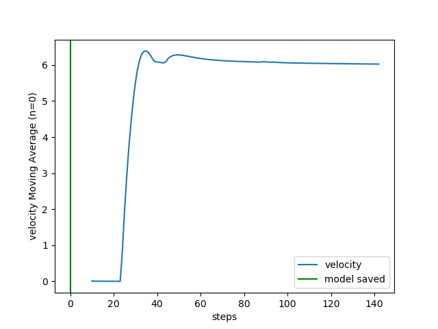
This change was sufficient to fix the throttle/brake issue, however, the performance of the agent was still bad. Couldn't even drive on straight roads. The reward plot was the following:


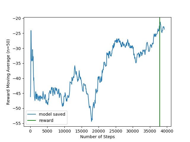
And an example of the driving is the following:


After some research, I realized the problem was the number of parameters of RegNet (4 milion). In every paper I read of Reinforcement Learning from pixels, the maximum number of parameters of the encoder was 1.5M.

Simple Encoder followed by SAC with longitudinal controller

To overcome the problem with the size of the encoder, I implemented a simple encoder with convolution layers - 1 million of parameters (issue #20). The reward plot looks much better:

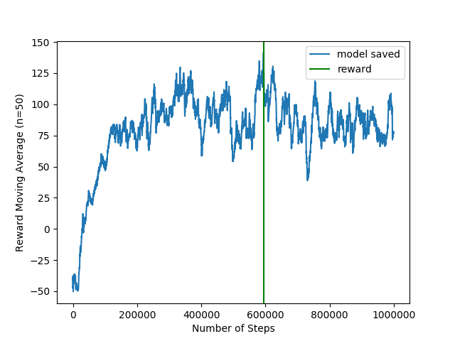
And the driving was also much better:



This architecture will be referred to as the baseline architecture in this blog. The baseline architecture was then tested on Corl2017 benchmark in the navigation task:

Agent	Score Route	Score Penalty	Score Composed
Baseline	0.27	0.69	0.19

Adding Data Augmentation to the baseline architecture

Following this paper, everytime a batch size was sampled from the memory of the agent, a random crop was applied to the images (issue #7). The authors claimed that this data augmentation serve as a regularizer, making the learning process more stable.

The reward plot of this method was the following:

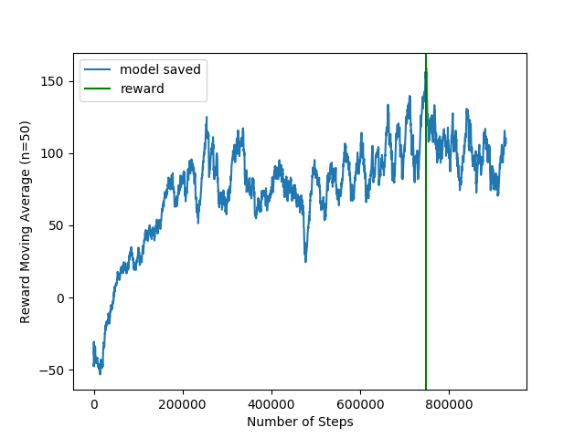
And now the performance on Corl2017-navigation:

Agent	Score Route	Score Penalty	Score Composed
Baseline	0.27	0.69	0.19
Augmentation	0.24	0.67	0.17

The results using Augmentation are worse than our baseline, which could indicate that this data augmentation technique is not suitable for autonomous driving, or that the data augmentation in general does not have much impact on autonomous driving.

Adding AutoEncoder to the baseline architecture

Following this paper, I implemented an AutoEncoder as an additional loss to force the compact representation of the images to contain relevant information about the image itself (issue #23). The architecture is the following:

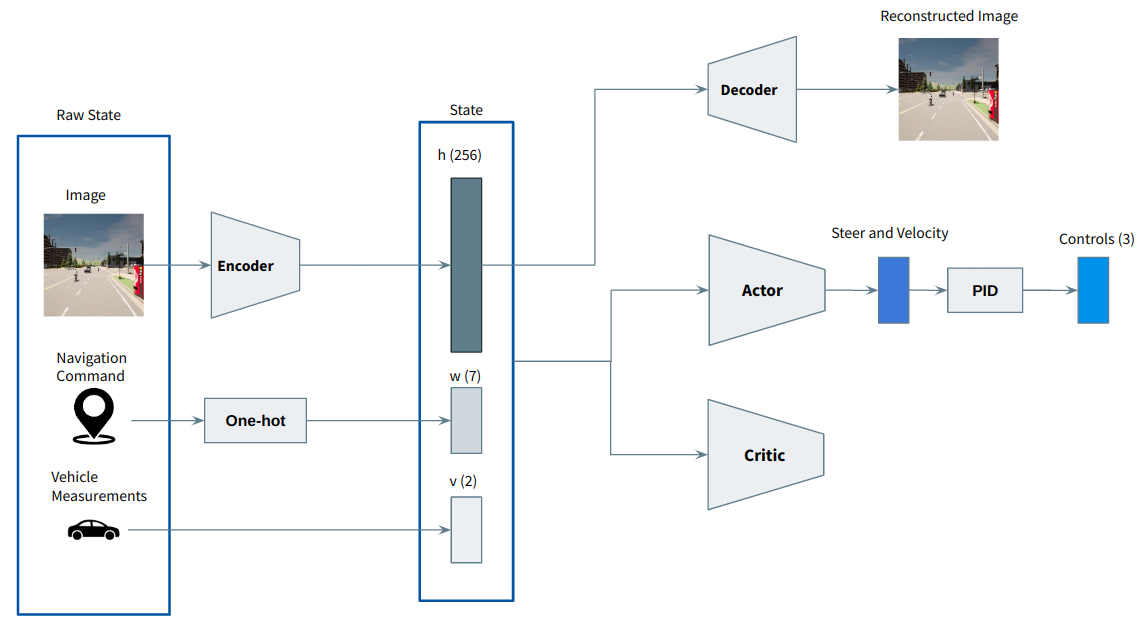
Once the training was over, I gave the following image to the system:



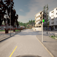
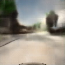
And the reconstructed image was the following:

The reward plot is the following:

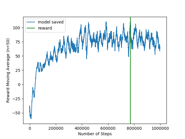
And the performace is:

Agent	Score Route	Score Penalty	Score Composed
Baseline	0.27	0.69	0.19
Augmentation	0.24	0.67	0.17
AutoEncoder	0.21	0.67	0.15

And once again, the results are worse than the baseline. There are some examples in the literature that claim that the reconstruction of the input image alone is insufficient to improve the performance of the agent. In autonomous driving, it is common to reconstruct the segmented image instead of the raw image, which is something I expect to test in the future.

What's Next?

In the next month I'll continue working on implementing techniques to improve the sample efficiency, namely: contrastive learning and DDPG with sigma decaying.

In addition, I expect to introduce temporal information into the system using two different approaches: a) by concatenating the different images and b) by using recurrent networks.